Current page:

Optimization and optimal control

These notes were originally written by T. Bretl and were transcribed by S. Bout.

Optimization

The following thing is called an optimization problem:

The solution to this problem is the value of that makes as small as possible.

We know that we are supposed to choose a value of because "" appears underneath the “minimize” statement. We call the decision variable.
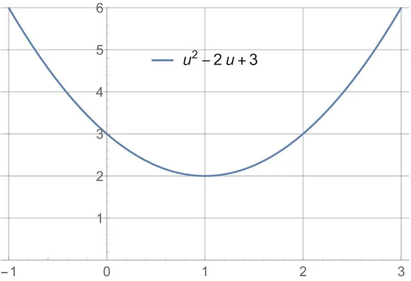
We know that we are supposed to minimize because "" appears to the right of the “minimize” statement. We call the cost function.

In particular, the solution to this problem is . There are at least two different ways to arrive at this result:

We could plot the cost function. It is clear from the plot that the minimum is at .
We could apply the first derivative test. We compute the first derivative:

Then, we set the first derivative equal to zero and solve for :

Values of that satisfy the first derivative test are only “candidates” for optimality — they could be maxima instead of minima, or could be only one of many minima. We’ll ignore this distinction for now. Here’s a plot of the cost function and of it’s derivative. Note that, clearly, the derivative is equal to zero when the cost function is minimized: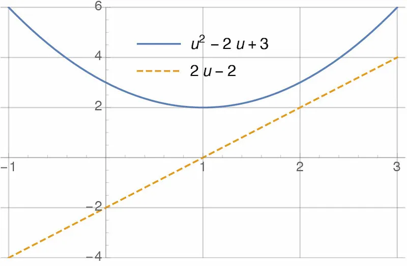

In general, we write optimization problems like this:

Again, is the decision variable and is the cost function. In the previous example:

Here is another example:

The solution to this problem is the value of both and that, together, make

as small as possible. There are two differences between this optimization problem and the previous one. First, there is a different cost function:

Second, there are two decision variables instead of one. But again, there are at least two ways of finding the solution to this problem:

We could plot the cost function. The plot is now 3D — the “x” and “y” axes are and , and the “z” axis is . The shape of the plot is a bowl. It’s hard to tell where the minimum is from looking at the bowl, so I’ve also plotted contours of the cost function underneath. “Contours” are like the lines on a topographic map. From the contours, it looks like the minimum is at .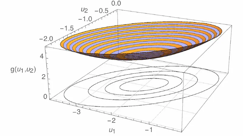
We could apply the first derivative test. We compute the partial derivative of with respect to both and :

Then, we set both partial derivatives equal to zero and solve for and :

As before, we would have to apply a further test in order to verify that this choice of is actually a minimum. But it is certainly consistent with what we observed above. Here is a plot of each partial derivative as a function of and . The shape of each plot is a plane (i.e., a flat surface). Both planes are zero at :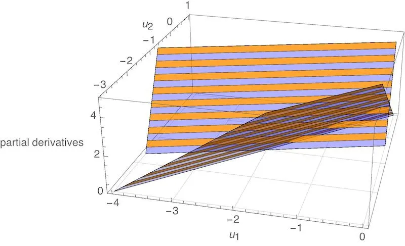

An equivalent way of stating this same optimization problem would have been as follows:

You can check that the cost function shown above is the same as the cost function we saw before (e.g., by multiplying it out). We could have gone farther and stated the problem as follows:

We have returned to having just one decision variable , as in the first example, but this variable is now a matrix — i.e., it has two elements, which we would normally write as and . The point here is that the “decision variable” in an optimization problem can be a variety of different things: a scalar, a vector (i.e., an matrix), and — as we will see — even a function of time. Before proceeding, however, let’s look at one more example of an optimization problem:

This example is exactly the same as the previous example, except that the two decision variables (now renamed and ) are subject to a constraint:

We are no longer free to choose and arbitrarily. We are restricted to choices that satisfy the constraint. The solution to this optimization problem is the value that minimizes the cost function, chosen from among all values that satisfy the constraint. Again, there are a variety of ways to solve this problem. One way is to eliminate the constraint. First, we solve the constraint equation:

Then, we plug this result into the cost function:

By doing so, we have shown that solving the constrained optimization problem

is equivalent to solving the unconstrained optimization problem

and then taking . We can do so easily by taking the first derivative and setting it equal to zero, as we did in the first example:

The point here was not to show how to solve constrained optimization problems in general, but rather to identify the different parts of a problem of this type. As a quick note, you will sometimes see the example optimization problem we’ve been considering written as

The meaning is exactly the same, but isn’t listed as one of the decision variables under “minimize.” The idea here is that is an “extra variable” that we don’t really care about. This optimization problem is trying to say the following:

“Among all choices of for which there exists an satisfying , find the one that minimizes .”

Minimum vs. Minimizer

We have seen three example problems. In each case, we were looking for the minimizer, i.e., the choice of decision variable that made the cost function as small as possible:

The solution to

was .
The solution to

was .
The solution to

was .

It is sometimes useful to focus on the minimum instead of on the minimizer, i.e., what the “smallest value” was that we were able to achieve. When focusing on the minimum, we often use the following “set notation” instead:

The problem

is rewritten

The meaning is to “find the minimum value of over all choices of .” The solution to this problem can be found by plugging in what we already know is the minimizer, . In particular, we find that the solution is .
The problem

is rewritten

Again, the meaning is to “find the minimum value of over all choices of and .” We plug in what we already know is the minimizer to find the solution — it is .
The problem

is rewritten

And again, the meaning is to “find the minimum value of over all choices of for which there exists satisfying .” Plug in the known minimizer, , and we find that the solution is 15.

The important thing here is to understand the notation and to understand the difference between a “minimum” and a “minimizer.”

Optimal Control

Statement of the problem

The following thing is called an optimal control problem:

Let’s try to understand what it means.

The statement

says that we are being asked to choose an input trajectory that minimizes something. Unlike in the optimization problems we saw before, the decision variable in this problem is a function of time. The notation is one way of indicating this. Given an initial time and a final time , we are being asked to choose the value of at all times in between, i.e., for all .
The statement

is a constraint. It implies that we are restricted to choices of for which there exists an satisfying a given initial condition

and satisfying the ordinary differential equation

One example of an ordinary differential equation that looks like this is our usual description of a system in state-space form:
The statement

says what we are trying to minimize — it is the cost function in this problem. Notice that the cost function depends on both and . Part of it, , is integrated (i.e., “added up”) over time. Part of it, , is applied only at the final time. One example of a cost function that looks like this is

The HJB equation (our new “first-derivative test”)

As usual, there are a variety of ways to solve an optimal control problem. One way is by application of what is called the Hamilton-Jacobi-Bellman Equation, or “HJB.” This equation is to optimal control what the first-derivative test is to optimization. To derive it, we will first rewrite the optimal control problem in “minimum form” (see “Minimum vs Minimizer”):

Nothing has changed here, we’re just asking for the minimum and not the minimizer. Next, rather than solve this problem outright, we will first state a slightly different problem:

The two changes that I made to go from the original problem to this one are:

Make the initial time arbitrary (calling it instead of ).
Make the initial state arbitrary (calling it instead of ).

I also made three changes in notation. First, I switched from to to avoid getting confused between as initial condition and as state trajectory. Second, I switched from to to be consistent with the switch from to . Third, I switched from calling time to calling time to avoid getting confused with my use of as a name for the initial time.

You should think of the problem (2) as a function itself. In goes an initial time and an initial state , and out comes a minimum value. We can make this explicit by writing

We call the value function. Notice that is the solution to the original optimal control problem that we wanted to solve — the one where the initial time is and the initial state is . More importantly, notice that satisfies the following recursion:

The reason this equation is called a “recursion” is that it expresses the function in terms of itself. In particular, it splits the optimal control problem into two parts. The first part is from time to time . The second part is from time to time . The recursion says that the minimum value is the sum of the cost

from the first part and the cost

from the second part (where "" is whatever the state turns out to be, starting at time from start and applying the input ), which we recognize as the definition of

We now proceed to approximate the terms in (4) by first-order series expansions. In particular, we have

and we also have

If we plug both of these into (4), we find

Notice that nothing inside the minimum depends on anything other than , , and . So we can drop the constraint and make the only decision variable. In fact, we might as well replace simply by "" since we only care about the input at a single instant in time:

Also, notice that

does not depend on , so it can be brought out of the minimum:

To simplify further, we can subtract from both sides, then divide everything by :

The equation is called the Hamilton-Jacobi-Bellman Equation, or simply the HJB equation. As you can see, it is a partial differential equation, so it needs a boundary condition. This is easy to obtain. In particular, going all the way back to the definition (3), we find that

The importance of HJB is that if you can find a solution to (5)-(6) — that is, if you can find a function that satisfies the partial differential equation (5) and the boundary condition (6) — then the minimizer in (5), evaluated at every time , is the solution to the optimal control problem (1). You might object that (5) “came out of nowhere.” First of all, it didn’t. We derived it just now, from scratch. Second of all, where did the first-derivative test come from? Could you derive that from scratch? (Do you, every time you need to use it? Or do you just use it?)

Solution approach

The optimal control problem

can be solved in two steps:

Find :
Find :

LQR

Statement of the problem

Here is the linear quadratic regulator (LQR) problem:

It is an optimal control problem — if you define

then you see that this problem has the same form as (1). It is called “linear” because the dynamics are those of a linear (state space) system. It is called “quadratic” because the cost is quadratic (i.e., polynomial of order at most two) in and . It is called a “regulator” because the result of solving it is to keep close to zero (i.e., to keep errors small).

The matrices , , and are parameters that can be used to trade off error (non-zero states) with effort (non-zero inputs). These matrices have to be symmetric (, etc.), have to be the right size, and also have to satisfy the following conditions in order for the LQR problem to have a solution:

What this notation means is that and are positive semidefinite and that is positive definite (see wikipedia). We will ignore these terms for now, noting only that this is similar to requiring (for example) that in order for the function to have a minimum.

Do the matrices Q, R, and M really have to be symmetric?

Suppose is not symmetric. Define

First, notice that is symmetric:

In fact, — when defined in this way — is often referred to as the symmetric part of .

Second, notice that we can replace with without changing the cost:

So, it is not that , , and “have to be” symmetric, it’s that they “might as well be” symmetric — if they’re not, we can replace them with matrices that are symmetric without changing the cost.

Solution to the problem

Our “Solution approach” tells us to solve the LQR problem in two steps. First, we find a function that satisfies the HJB equation. Here is that equation, with the functions , , and filled in from our “Statement of the problem”:

What function might solve this equation? Look at the boundary condition. At time ,

This function has the form

for some symmetric matrix that satisfies . So let’s “guess” that this form is the solution we are looking for, and see if it satisfies the HJB equation. Before proceeding, we need to compute the partial derivatives of :

This is matrix calculus (e.g., see wikipedia or Chapter A.4.1 of Convex Optimization (Boyd and Vandenberghe)). The result on the left should surprise no one. The result on the right is the matrix equivalent of

You could check that this result is correct by considering an example. Plug these partial derivatives into HJB and we have

To evaluate the minimum, we apply the first-derivative test (more matrix calculus!):

This equation is easily solved:

Plugging this back into (7), we have

In order for this equation to be true for any , it must be the case that

In summary, we have found that

solves the HJB equation, where is found by integrating the matrix differential equation

backward in time, starting from

Now that we know , we can find . Wait, we already did that! The minimizer in the HJB equation is (8). This choice of input has the form

for

LQR Code

Here is how to find the solution to an LQR problem with Python:

Text successfully copied to clipboard!

import numpy as np
from scipy import linalg

def lqr(A, B, Q, R):
    # Find the cost matrix
    P = linalg.solve_continuous_are(A, B, Q, R)
    # Find the gain matrix
    K = linalg.inv(R) @ B.T @ P
    return K