Equations of Motion of a 2-DOF Planar Robotic Manipulator

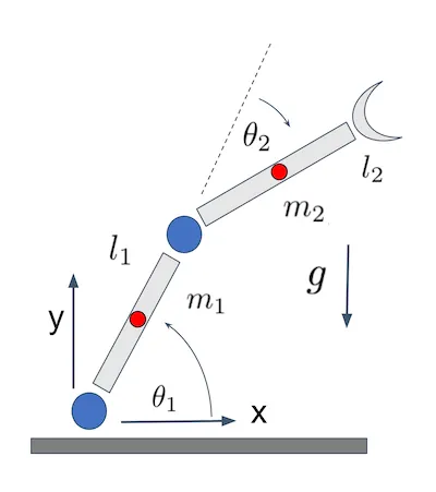
Kinematics for the Robot Arm Links

The position of the center of mass of the first link reads

where encodes the location of the center of mass of link 1. For instance, , if the link is symmetric and has uniform density. The equations relate the Cartesian coordinates of to the first generalized coordinate . The position of the second link center of mass can be calculated via

which accounts for the fact that the second arm is attached to the first and that we have another generalized coordinate, , the second joint angle measured with respect to the orientation of the first link. Once again, , if the center of mass is at the midpoint of the link. The above equations are sufficient to describe the translational kinematics of the robot arm. However, we also need to consider rotational kinematics.

Kinetic and Potential Energy

In order to construct the Lagrangian we need to determine the kinetic () and potential energy () of the system. The total kinetic energy can be expressed as the sum of the rotational and translational kinetic energy

Here, the squared velocities of the centers of mass of both links via , ,

Since we also consider rotational kinematics we have to account for the change in the kinetic energy due to the rotation of each link about its center of mass. The corresponding angular velocities read

The potential energy is:

Euler Lagrange Equations

The main idea is that the Euler–Lagrange equations result in the equations of motion for the links. To control that motion, external torques are required which modify the joint angles .

where is the above Lagrangian. The resulting equations are often expressed in the following form

where is the so-called Mass matrix or Inertia Matrix that generally depends on the configuration of the arm, are the Coriolis and Centrifugal Term which depend on the velocity of the joint angles and the Gravity Terms are collected in G. The torques, in this example , constitute the external input.

The Inertia Matrix

In our example of a two link robotic arm, we have two generalized coordinates

and thus the inertia matrix consists of 4 elements:

Those are

Note that this matrix changes with the configuration of the robotic arm.

Coriolis and Centrifugal Terms

A common form of the velocity-dependent matrix is:

where . This means the matrix is traceless, and the inner product is a vector of the form

Gravity Terms

The remaining terms are due to gravity and are collected in . Since , we find

Final Equations of Motion

The final equations of motion read

Trajectory Planning

To move the robotic arm smoothly from its initial configuration to the target configuration, we plan trajectories for the joint angles and over time and calculate the torques and that enable such motion.
A common, even though somewhat counterintuitive approach is not to solve the equations of motion for the joint angles but to assert that all angles must behave in a way that smooths transitions between the initial and final positions. In other words, we postulate that a joint angle must be representable through a cubic polynomial:

The coefficients are computed from boundary conditions (initial/final positions, velocities, and optionally accelerations).

The time evolution of the joint angles is given by

and angular velocities and accelerations follow by differentiation:

With the joint velocities and accelerations known, the required joint torques and are computed using the inverse dynamics equation

by substituting for their corresponding polynomials.

Numerical Example

Let us consider the an example with the following parameters:

• Link lengths: ,
• Initial end-effector position: ,
• Desired end-effector position: ,
• ,
• , ,
• , the gravitational acceleration on Earth at sea-level
• ,

where is the total time it takes the end-effector to reach its target configuration.

Step 1: Solve the Inverse Kinematics

First we need to calculate the value of the generalized coordinates at the initial and final times. To achieve the desired end-effector position , we solve the inverse kinematics problem to find the joint angles and . From the end-effector position equations

we can derive

and find the joint angles and required to achieve the target end-effector position

Here, is the quadrant corrected arctangent. Inserting numerical values for and we find

Step 2: Boundary Conditions

Suppose we plan to reach the target configuration in seconds, starting from rest.
Then, based on the inverse Kinematics we have

Since we also want the arm to be at rest before and after the maneuver we add

where all values have units of rad/s.

Step 3: Compute Velocities and Accelerations

The joint angles should follow a cubic polynomial trajectory:

From the boundary conditions we can compute the coefficients for and . Let us start with . The boundary conditions imply that

The boundary conditions and result in

Since we know we can solve for the coefficients

in units of rad/s and rad/s, respectively.

Following a similar path, we find the coefficients for

The final equations for the joint angles and their derivatives in units of rad, rad/s and rad/s read

Step 4: Compute Required Torques

We can now compute the torques and by substituting the constants into the equations of motion

This results in

Inserting the polynomials for finally lets us write the required torques as function of time in units of Nm